Modelling metapopulations

Background

aae.pop has a built-in method to define a metapopulation from multiple populations. This is based on the most-general definition of a metapopulation: populations of the same species connected by dispersal. Defining a metapopulation requires dynamics objects for multiple populations, a structure that defines movements between populations, and a dispersal object, which is a new class of object used to specify in detail the movements between populations.

This vignette introduces structure and dispersal objects and explains how population processes (e.g., demographic stochasticity) are handled in metapopulations.

Defining a metapopulation

Simulating metapopulation dynamics is very similar to the basic simulate approach outlined in the Getting started vignette. The only difference is that the population matrix has to be expanded to include multiple populations and movements among these populations. This section will start with a highly simplified example of a building a metapopulation from scratch and will then introduce some methods in aae.pop to streamline this process for more realistic population models.

First, define a simplistic two-class model:

popmat_simple <- matrix(
  c(
    0, 2,       # reproduction of 10 new individuals per adult (female)
    0.45, 0.15  # move from class 1 to class 2 with 0.8 probability,
                # survive in class 2 with 0.25 probability
  ),
  nrow = 2,
  byrow = TRUE
)

If we assume there are two separate populations with same underlying vital rates (defined in popmat_simple), it is possible to build up a four-class model that has two classes from population 1 and another two classes from population 2:

# setup a matrix with four classes and all elements equal to zero
metapop_simple <- matrix(0, nrow = 4, ncol = 4)

# fill the first population's vital rates
#   (top two rows, two left-hand columns)
metapop_simple[1:2, 1:2] <- popmat_simple

# repeat for the second population, this time
#   filling the bottom right square
metapop_simple[3:4, 3:4] <- popmat_simple

This matrix defines transitions between all four classes (two classes each in two populations), but currently keeps transitions within populations. Following the columns move to rows rule of aae.pop, the metapop_simple matrix defines transitions from class 1 to class 2, class 2 to classes 1 and 2, class 3 to class 4, and class 4 to classes 3 and 4:

##      [,1] [,2] [,3] [,4]
## [1,] 0.00 2.00 0.00 0.00
## [2,] 0.45 0.15 0.00 0.00
## [3,] 0.00 0.00 0.00 2.00
## [4,] 0.00 0.00 0.45 0.15

Adding dispersal, or movement between the two populations, requires transitions from class 1 or 2 to class 3 or 4, and vice versa. For example, dispersal might be a feature of the second class only (adults), in which case individuals would move between class 2 and class 4. These movements will be defined by cells [2, 4] and [4, 2] in metapop_simple:

# allow 30 % of surviving adults to move between populations
#   (columns move to rows, so population 1 to 2 is in [4, 2] and
#    population 2 to 1 is in [2, 4])
metapop_simple[4, 2] <- 0.3 * metapop_simple[2, 2]
metapop_simple[2, 4] <- 0.3 * metapop_simple[4, 4]

# this 30 % needs to be removed from the adults that survive
#   and remain within the same population
metapop_simple[2, 2] <- metapop_simple[2, 2] - metapop_simple[4, 2]
metapop_simple[4, 4] <- metapop_simple[4, 4] - metapop_simple[2, 4]

# what happens if we simulate from this?
sims <- simulate(dynamics(metapop_simple), nsim = 100)
plot(sims, col = scales::alpha("#2171B5", 0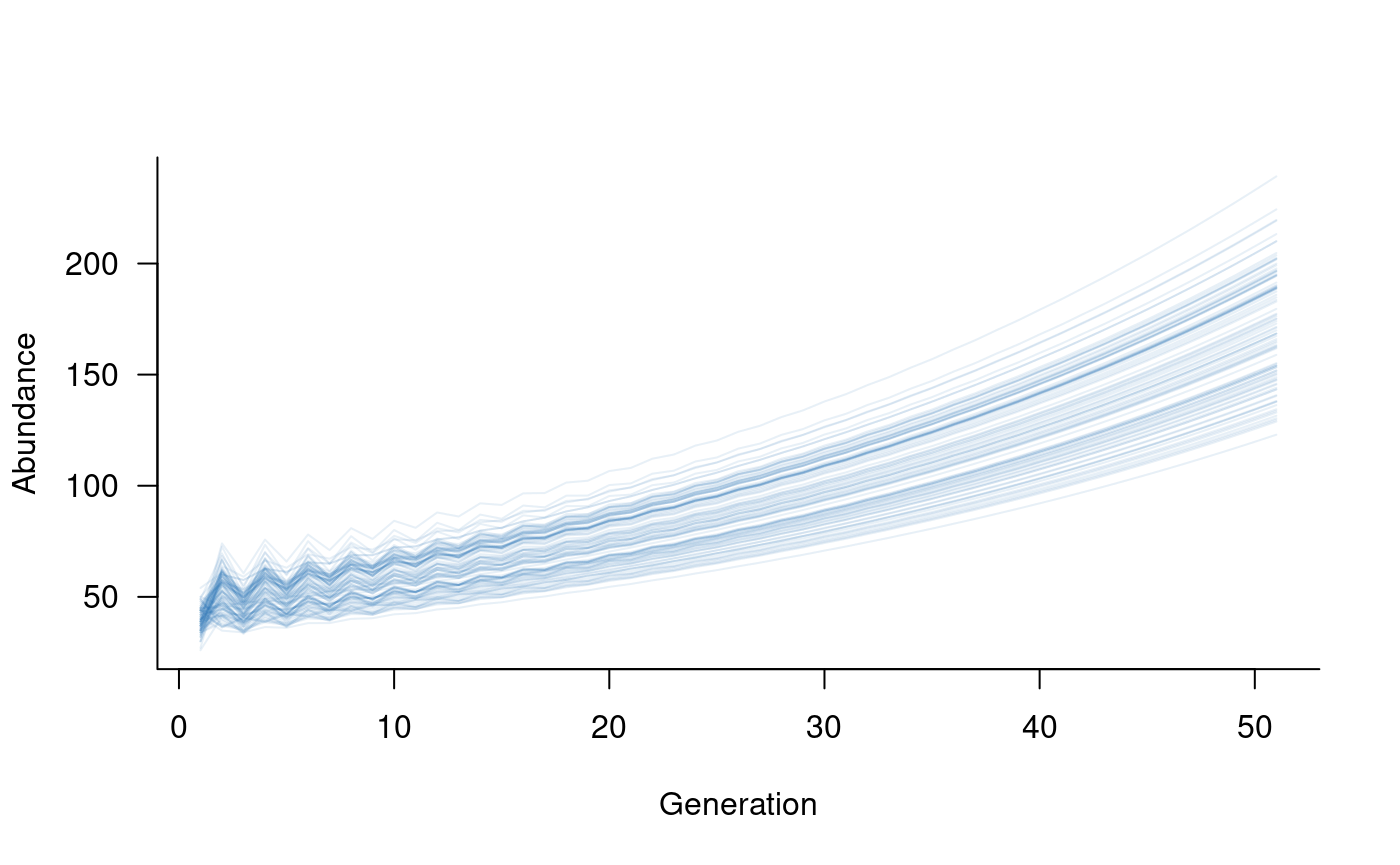.1))

This plot sums over both populations, which is often of interest when considering species- or metapopulation-level abundances. aae.pop has a built-in subset method, which means it’s possible to separate the two populations, recalling that population 1 is classes 1 and 2 and population 2 is classes 3 and 4 in the population vector:

pop1_sims <- subset(sims, 1:2)
pop2_sims <- subset(sims, 3:4)
plot(pop1_sims, col = scales::alpha("#2171B5", 0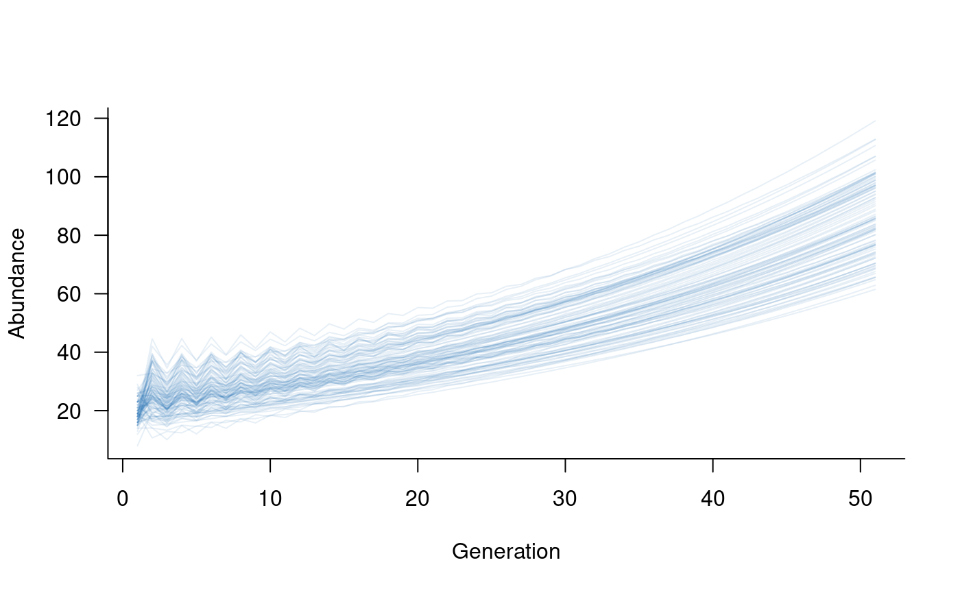.1))

plot(pop2_sims, col = scales::alpha("#2171B5", 0.1))

This illustrates a highly simplified metapopulation model, highlighting the main steps in its construction: define population dynamics of each separate population, define dispersal among populations, and account for the effects of dispersal on within-population vital rates. The following sections outline how these steps are generalised in aae.pop to deal with realistically complex models.

Structure

The structure of a metapopulation defines how populations are connected. Structure is captured in aae.pop by a matrix of zeros and ones that denote links between two populations. This matrix has one row and one column for each population, and follows the same columns move to rows rule as the population matrix. For example, a 1 in the second row, first column, indicates that individuals from population 1 can move to population 2. A 1 in the first row, second column denotes the reverse movement (population 2 to population 1).

For the simplistic example above, the structure would look like:

##      [,1] [,2]
## [1,]    0    1
## [2,]    1    0

This structure can be defined as:

structure_simple <- matrix(c(0, 1, 1, 0), nrow = 2)

Increasing the number of populations is a direct extension of this approach. With five populations all connected by dispersal, the structure would look like:

##      [,1] [,2] [,3] [,4] [,5]
## [1,]    0    1    1    1    1
## [2,]    1    0    1    1    1
## [3,]    1    1    0    1    1
## [4,]    1    1    1    0    1
## [5,]    1    1    1    1    0

A more realistic structure might consider five populations with only some of these possible connections, which might look like:

##      [,1] [,2] [,3] [,4] [,5]
## [1,]    0    1    0    0    0
## [2,]    0    0    0    1    0
## [3,]    1    1    0    0    0
## [4,]    1    0    0    0    0
## [5,]    0    0    0    1    0

In this example, individuals from population 1 move to populations 3 and 4, individuals from population 2 move to populations 1 and 3, and individuals from population 4 move to populations 2 and 5. Individuals from populations 3 and 5 never move to other populations.

Dispersal

Defining the structure of a metapopulation is the first step towards simulating metapopulation dynamics. However, this definition of structure is biologically vague. It specifies which populations are connected and the direction of those connections, but doesn’t specify which classes within populations are moving and how frequently. dispersal objects specify the probability of a transition between specific source and receiver classes, whether these transitions are density dependent, and any stochasticity in the transitions. dispersal objects are one-directional, which means a separate dispersal object is required for each link in the structure matrix.

Using the simplistic, two-class example, which had adults moving both directions between the two populations, the dispersal objects could be specified as:

kern <- matrix(c(0, 0, 0, 0.3), nrow = 2)
dispersal_simple <- dispersal(kernel = kern, proportion = TRUE)

The kernel is a matrix with two rows and two columns, and the 0.3 in the bottom-right corner specifies the 30 % of surviving adults that move from one population to another. The argument proportion determines whether this 30 % of moving individuals is a proportion of all surviving adults or is an absolute value. Setting proportion = TRUE addresses the situation where the 30 % of moving adults are taken from the total pool of surviving adults, thereby reducing the within-population survival by 30 %.

This setup is sufficient to specify a one-direction movement between populations; an additional dispersal term is required to specify the reverse transition. In aae.pop, these dispersal terms can be combined in a list, stored in column-major order following the metapopulation structure. This means that one dispersal object must be provided for each link in the structure, working through the columns from left-to-right (i.e., all links in column 1, all links in column 2, and so on). In this simplistic example, the same dispersal term can be used for both links:

dispersal_simple <- list(dispersal_simple, dispersal_simple)

This example presents a simplified dispersal setup. aae.pop supports more complex features such as stochasticity and density dependence in transitions. These two extensions are discussed briefly below.

Putting it all together

Together, popmat_simple, structure_simple, and dispersal_simple are sufficient to characterise metapopulation dynamics as in metapop_simple. The metapopulation function ties these three elements together:

# create a population dynamics object from the population matrix
dynamics_simple <- dynamics(popmat_simple)

# turn this into a metapopulation
metapopulation_simple <- metapopulation(
  structure = structure_simple,
  dynamics = list(dynamics_simple, dynamics_simple), # both populations have identical rates
  dispersal = dispersal_simple
)

The metapopulation defined by metapopulation_simple is identical to that defined by metapop_simple, above:

all.equal(metapop_simple, metapopulation_simple$matrix)

## [1] TRUE

With metapopulation_simple defined in this way, simulating population dynamics is identical to any other population model in aae.pop:

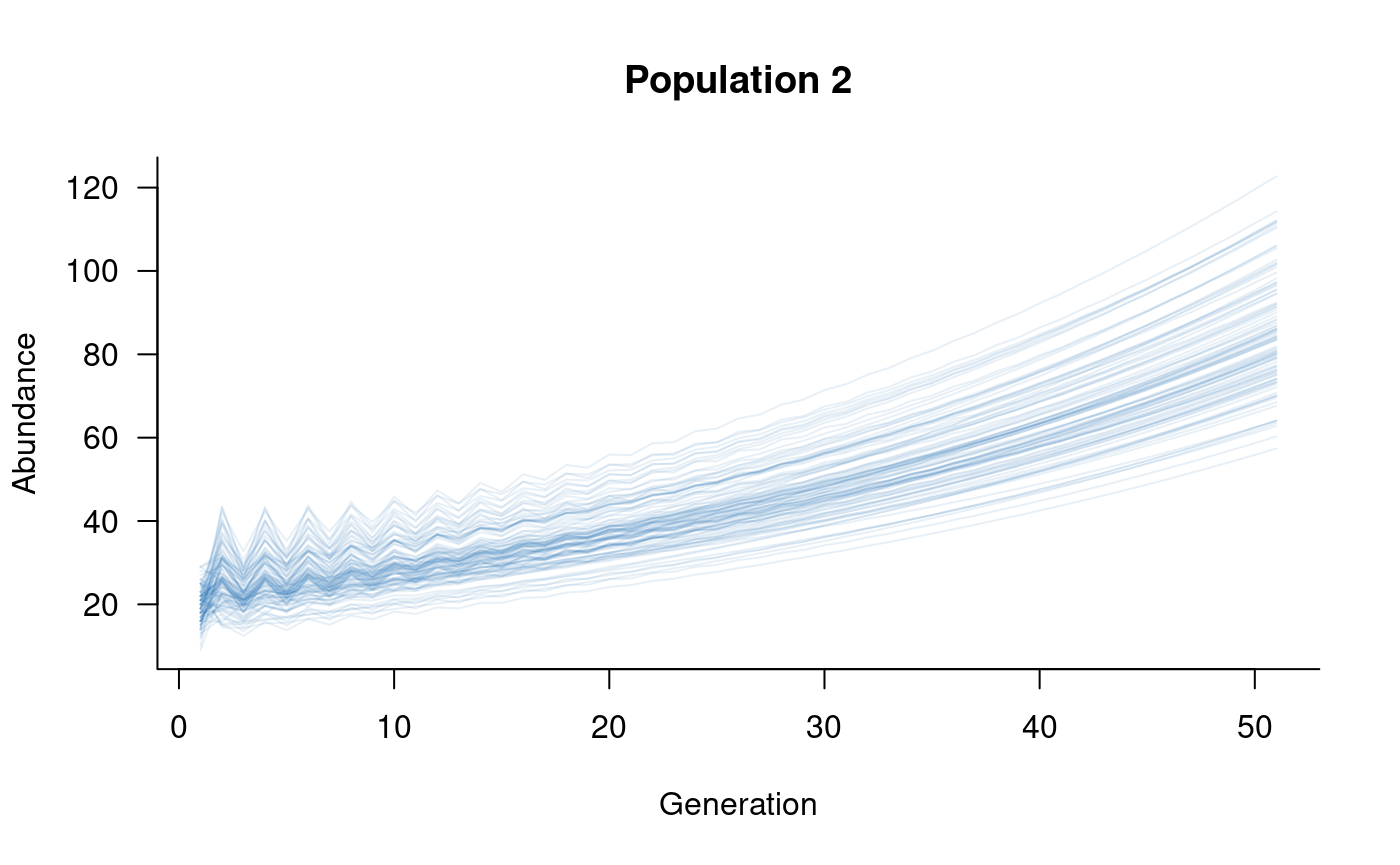
sims <- simulate(metapopulation_simple, nsim = 100)
plot(subset(sims, 1:2), col = scales::alpha("#2171B5", 0.1), main = "Population 1")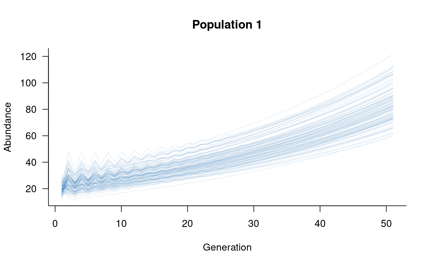

plot(subset(sims, 3:4), col = scales::alpha("#2171B5", 0.1), main = "Population 2")

A more complicated metapopulation structure might consider the population introduced in the Getting started vignette, which had five age classes. Coupling this with the five-population structure shown above demonstrates a more realistic metapopulation. Note that specifying this metapopulation manually would require a matrix with 25 rows and 25 columns, with each dispersal and proportional change in survival calculated individually. Using aae.pop still takes a few lines of code but many of the calculations are now handled automatically:

# define population matrix
popmat <- rbind(
  c(0,    0,    2,    4,    7),  # reproduction from 3-5 year olds
  c(0.25, 0,    0,    0,    0),  # survival from age 1 to 2
  c(0,    0.45, 0,    0,    0),  # survival from age 2 to 3
  c(0,    0,    0.70, 0,    0),  # survival from age 3 to 4
  c(0,    0,    0,    0.85, 0)   # survival from age 4 to 5
)

# define metapopulation structure
mp_str <- matrix(0, nrow = 5, ncol = 5)
mp_str[1, 2] <- mp_str[3, 2] <- mp_str[5, 4] <- mp_str[4, 1] <- mp_str[3, 1] <- mp_str[2, 4] <- 1

# define dispersal, assume all dispersal links are the same
mp_kern <- matrix(0, nrow = 5, ncol = 5)
mp_kern[3, 4] <- mp_kern[4, 5] <- 0.2  # adults can move once per year with 20 % probability
mp_disp <- dispersal(kernel = mp_kern, proportion = TRUE)

# define metapopulation
mp <- metapopulation(
  structure = mp_str,
  dynamics = lapply(1:5, function(x) dynamics(popmat)),   # five populations, all identical rates
  dispersal = lapply(1:6, function(x) mp_disp)  # six transitions in mp_str, all identical
)

# simulate
sims <- simulate(mp, nsim = 100)

# plot
plot(sims, col = scales::alpha("#2171B5", 0.1), main = "All populations")

With five populations, each with five classes, the simulated values now have 25 total classes. These are stored in order of the five populations defined in the dynamics argument to metapopulation, so classes 1 to 5 are the first population, 6 to 10 are the second population, and so on. These can be extracted and plotted with the subset function:

plot(subset(sims, 1:5), col = scales::alpha("#2171B5", 0.1), main = "Population 1")

plot(subset(sims, 21:25), col = scales::alpha("#2171B5", 0.1), main = "Population 5")

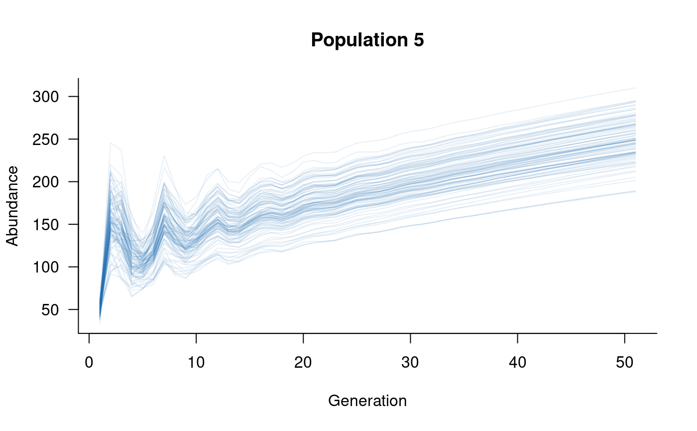
These plots illustrate the effects of metapopulation dynamics: population 1 loses more individuals than it gains and is in decline, whereas population 5 only gains individuals and is on an upward trajectory as a result.

What happens to within-population processes?

The metapopulation function preserves all within-population processes, such as density dependence, environmental and demographic stochasticity, and covariate effects (but see below for one complication with covariates). The processes operate within populations, so are largely separate from dispersal. Dispersal itself can be subject to among-population density dependence and stochasticity; this is described below.

Within-population processes are preserved using the same mask/function approach used for demographic processes, described in the Including processes vignette. A set of masks is created for each population (blocks on a block-diagonal matrix), and the functions for each population are coupled with the appropriate mask. This is an example of the flexibility of the mask/function approach.

A by-product of this setup is that processes (with the exception of dispersal) are assumed to be independent of all other populations. For example, density dependence will consider the number of individuals currently in a population but will not take into account the overall metapopulation abundance. If this level of detail is required, the metapopulation function could still be used to prepare the metapopulation-level elements (e.g., the metapopulation matrix, process functions), with additional processes added with metapopulation-level masks and functions (e.g., a new call to density_dependence).

A complication: covariates

The metapopulation function is designed to make metapopulation dynamics as similar as possible to single-population dynamics, which takes full advantage of the methods in simulate for (relatively) fast and flexible models. One complication is that simulate does not explicitly allow separate covariate sequences for each population. This is a relatively common scenario given that metapopulations typically span multiple spatial locations, and this section illustrates a possible workaround. An additional example of this approach is included in the metapopulation documentation (accessible by typing ?metapopulation into the R console). A more elegant solution is a focus for future development of aae.pop.

Using the simplified, two-population example above, this workaround involves combining two sequences of covariates into a single matrix (or data.frame), then subsetting this combined matrix within the covariates functions for each individual population.

# define two covariate sequences and combine them into a data.frame
covar_seq1 <- runif(20, min = 0.5, max = 1.0)
covar_seq2 <- runif(20, min = 0.75, max = 1.0)
covar_seq <- data.frame(pop1 = covar_seq1, pop2 = covar_seq2)

# define covariate responses for each population, pulling out
#   the appropriate covariate sequence in each
covar_fn1 <- function(mat, x) {
  mat * x$pop1
}
covar_fn2 <- function(mat, x) {
  mat * x$pop2
}

# define the covariates object for each population
covar1 <- covariates(masks = transition(popmat_simple), funs = covar_fn1)
covar2 <- covariates(masks = transition(popmat_simple), funs = covar_fn2)

# create a population dynamics object for each population
dynamics_simple1 <- dynamics(popmat_simple, covar1)
dynamics_simple2 <- dynamics(popmat_simple, covar2)

# turn this into a metapopulation
metapopulation_simple <- metapopulation(
  structure = structure_simple,
  dynamics = list(dynamics_simple1, dynamics_simple2),
  dispersal = dispersal_simple
)

# simulate
sims <- simulate(
  metapopulation_simple,
  nsim = 100,
  args = list(covariates = format_covariates(covar_seq))
)

# plot
plot(sims, col = scales::alpha("#2171B5", 0.1), main = "Population-specific covariates")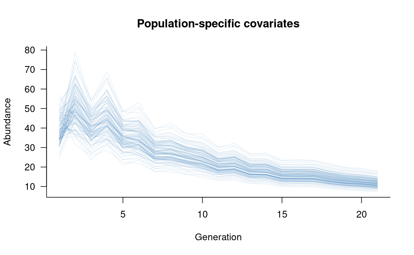

This example uses a named data.frame to store the covariate sequences for both populations but this approach could use any number of covariates and any form of subsetting or indexing of covariates within the covariate functions.

More on dispersal

The dispersal function, used above to define class-specific movements between two populations, also allows density dependence and stochasticity in these movements. These two processes are useful to account for scenarios where individual decisions to move depend on the number of individuals in the source or receiving population, and when outcomes of movement decisions are stochastic due to, for example, mortality risk during movement. Specification of density dependence and stochasticity in dispersal uses the same mask/function approach demonstrated in the Including processes vignette.

Stochasticity

It is highly likely that dispersal outcomes are stochastic due to unpredictable movements by individuals and increased mortality during and following dispersal. Stochasticity is supported in the definition of dispersal objects with a mask/function pair that identifies the relevant classes and form of stochasticity. Extending the simplified example from above, this might look like:

# define a mask that is TRUE whenever the dispersal kernel is non-zero
stoch_mask <- kern > 0

# define a stochastic dispersal function (small change in probability)
stoch_fun <- function(x) {
  rmultiunit(length(x), mean = x, sd = 0.05)
}

# using the kernel defined earlier (30 % probability of adults moving)
dispersal_simple <- dispersal(
  kernel = kern,
  stochasticity_masks = stoch_mask,
  stochasticity_funs = stoch_fun,
  proportion = TRUE
)

# dispersal is one-directional, so need one dispersal object for each population
dispersal_simple <- list(dispersal_simple, dispersal_simple)

# define metapopulation using the dynamics and structure objects defined above
metapopulation_simple <- metapopulation(
  structure = structure_simple,
  dynamics = list(dynamics_simple, dynamics_simple),
  dispersal = dispersal_simple
)

# simulate
sims <- simulate(metapopulation_simple, nsim = 100)

# plot
plot(sims, col = scales::alpha("#2171B5", 0.1), main = "Stochastic dispersal")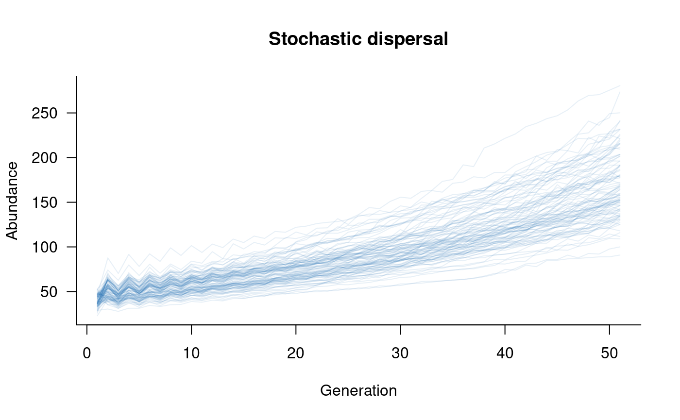

Density dependence

Density dependence might influence dispersal through individual decisions to move or remain based on the number of individuals in the current (source) or future (destination) population. More broadly, the abundances of source or destination populations might influence survival outcomes following dispersal due to levels of competition or other density-dependent stressors (e.g., disease). These types of processes can be included in a metapopulation model through the density_masks and density_funs arguments to dispersal.

The current implementation of density-dependent dispersal is linked the entire metapopulation vector, so can depend on the abundances of any or all of the sub-populations. The downside of this approach is that indexing of this vector has to be done manually in the definition of density_funs. This indexing depends on the order of populations within the metapopulation (as defined by the dynamics argument to metapopulation), recalling that each population has one element for each class. An example might illustrate the inclusion of density-dependent dispersal most clearly:

# define a mask that is TRUE whenever the dispersal kernel is non-zero
#   (this is the same as for stochasticity and this mask 
#    could be used for both)
dd_mask <- kern > 0

# define Ricker type density dependence based on the abundance in the
#    destination population (recall n is a vector of two classes per
#    population, so elements 1 and 2 are population 1 and elements
#    3 and 4 are population 2)
dd_fun1 <- function(x, n) {
  # dispersing from population 1 to 2
  x * exp(1 - sum(n[3:4]) / 20) / exp(1) 
}
dd_fun2 <- function(x, n) {
  # dispersing from population 2 to 1
  x * exp(1 - sum(n[1:2]) / 20) / exp(1)
}

# using the kernel defined earlier (30 % of surviving adults moving),
#    add density masks and functions for each population
dispersal_simple1 <- dispersal(
  kernel = kern,
  density_masks = dd_mask,
  density_funs = dd_fun1,
  proportion = TRUE
)
dispersal_simple2 <- dispersal(
  kernel = kern,
  density_masks = dd_mask,
  density_funs = dd_fun2,
  proportion = TRUE
)

# combine the dispersal objects for both populations
dispersal_simple <- list(dispersal_simple1, dispersal_simple2)

# define metapopulation using the dynamics and structure objects defined above
metapopulation_simple <- metapopulation(
  structure = structure_simple,
  dynamics = list(dynamics_simple, dynamics_simple),
  dispersal = dispersal_simple
)

# simulate
sims <- simulate(metapopulation_simple, nsim = 100)

# plot
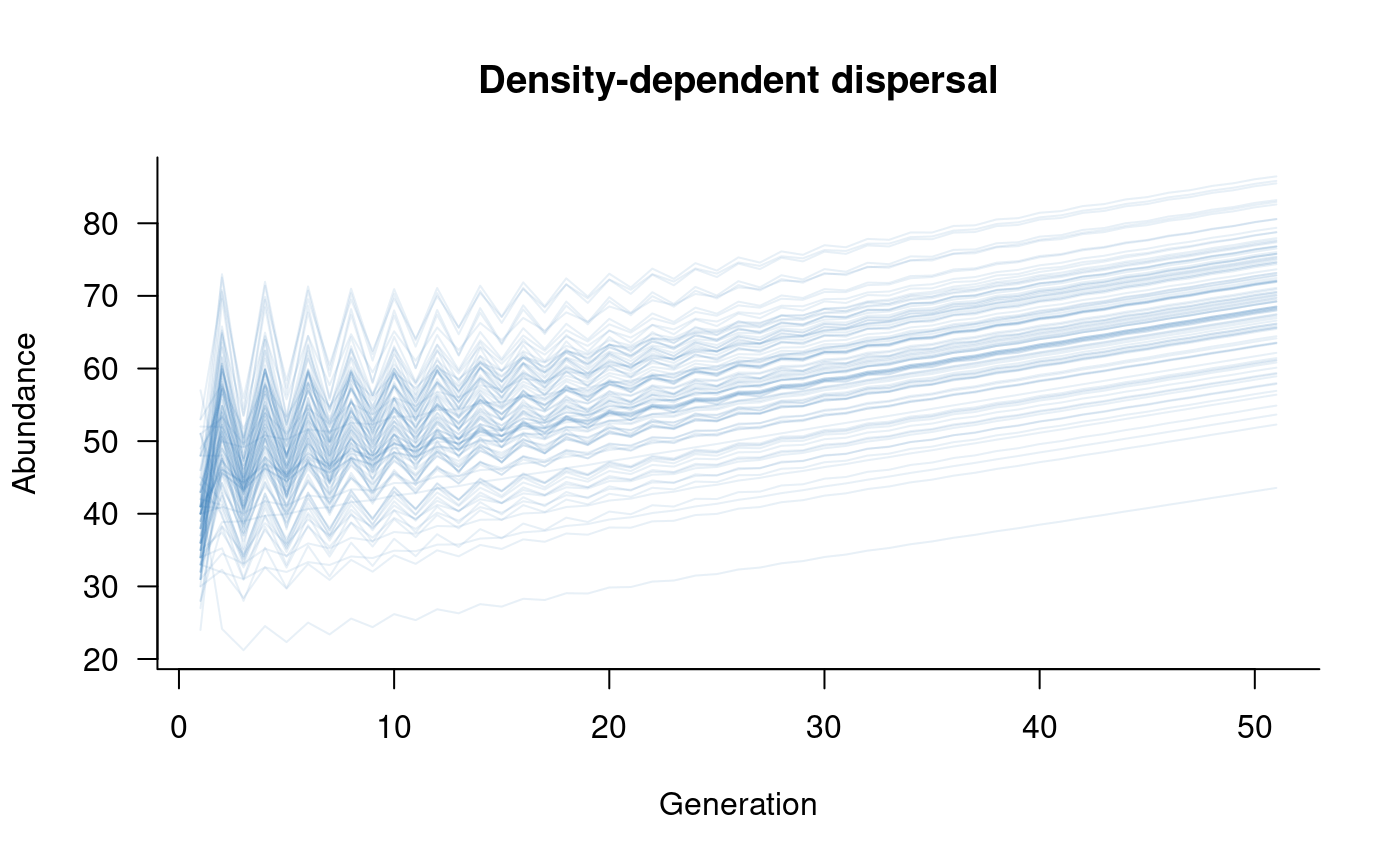
plot(sims, col = scales::alpha("#2171B5", 0.1), main = "Density-dependent dispersal")

Jian Yen

10/11/2020