Simulate single or multispecies population dynamics in R

Simulate population dynamics for one or more species defined by dynamics objects.

Usage

# S3 method for class 'dynamics'
simulate(
  object,
  nsim = 1,
  seed = NULL,
  ...,
  init = NULL,
  options = list(),
  args = list(),
  .future = FALSE
)

is.simulation(x)

is.simulation_list(x)

Arguments

object

a dynamics object created with dynamics or from a subsequent call to multispecies or metapopulation. Alternatively, object can be the output of a call to simulate in the case of summary

nsim

the number of replicate simulations (default = 1)

seed

optional seed used prior to initialisation and simulation to give reproducible results

...

ignored; included for consistency with simulate generic method

init

an array of initial conditions with one row per replicate and one column per population stage. If obj has been created with multispecies, initial conditions can be provided as a list or array with one element or slice per species, or as a matrix, in which case all species are assumed to share the same initial conditions. Defaults to NULL, in which case initial conditions are generated randomly according to options()$aae.pop_initialisation

options

a named list of simulation options. Currently accepted values are:

- ntime the number of time steps to simulate, ignored if obj includes a covariates (default = 50)

- keep_slices logical defining whether to keep intermediate population abundances or (if FALSE) to return only the final time slice

- tidy_abundances a function to handle predicted abundance data that may be non-integer. Defaults to identity; suggested alternatives are floor, round, or ceiling

- initialise_args a list of arguments passed to the function used to initialise abundance trajectories. Only used if init = NULL. Defaults to options()$aae.pop_lambda, which specifies lambda for Poisson random draws. The default initialisation function is defined by options()$aae.pop_initialisation.

- update a function to update abundances from one time step to the next. Defaults to options()$aae.pop_update.

args

named list of lists passing arguments to processes defined in object, including interaction for multispecies objects. Lists (up to one per process) can contain a mix of static, dynamic, and function arguments. Dynamic arguments must be lists with one element per time step. Function arguments must be functions that calculate arguments dynamically in each generation based on from the population dynamics object, population abundances, and time step in each generation. All other classes (e.g., single values, matrices, data frames) are treated as static arguments. Covariates contained in numeric vectors, matrices, or data frames can be formatted as dynamic arguments with the format_covariates function.

args for multispecies objects must have one element per species (defaults will expand automatically if not provided)

.future

flag to determine whether the future package should be used to manage updates for multispecies models (an embarrassingly parallel problem)

x

an object to pass to is.simulation or is.simulation.list

Details

Includes plot and subset methods

Examples

# define a population matrix (columns move to rows)
nclass <- 5
popmat <- matrix(0, nrow = nclass, ncol = nclass)
popmat[reproduction(popmat, dims = 4:5)] <- c(10, 20)
popmat[transition(popmat)] <- c(0.25, 0.3, 0.5, 0.65)

# can extract standard population matrix summary stats
lambda <- Re(eigen(popmat)$values[1])

# define a dynamics object
dyn <- dynamics(popmat)

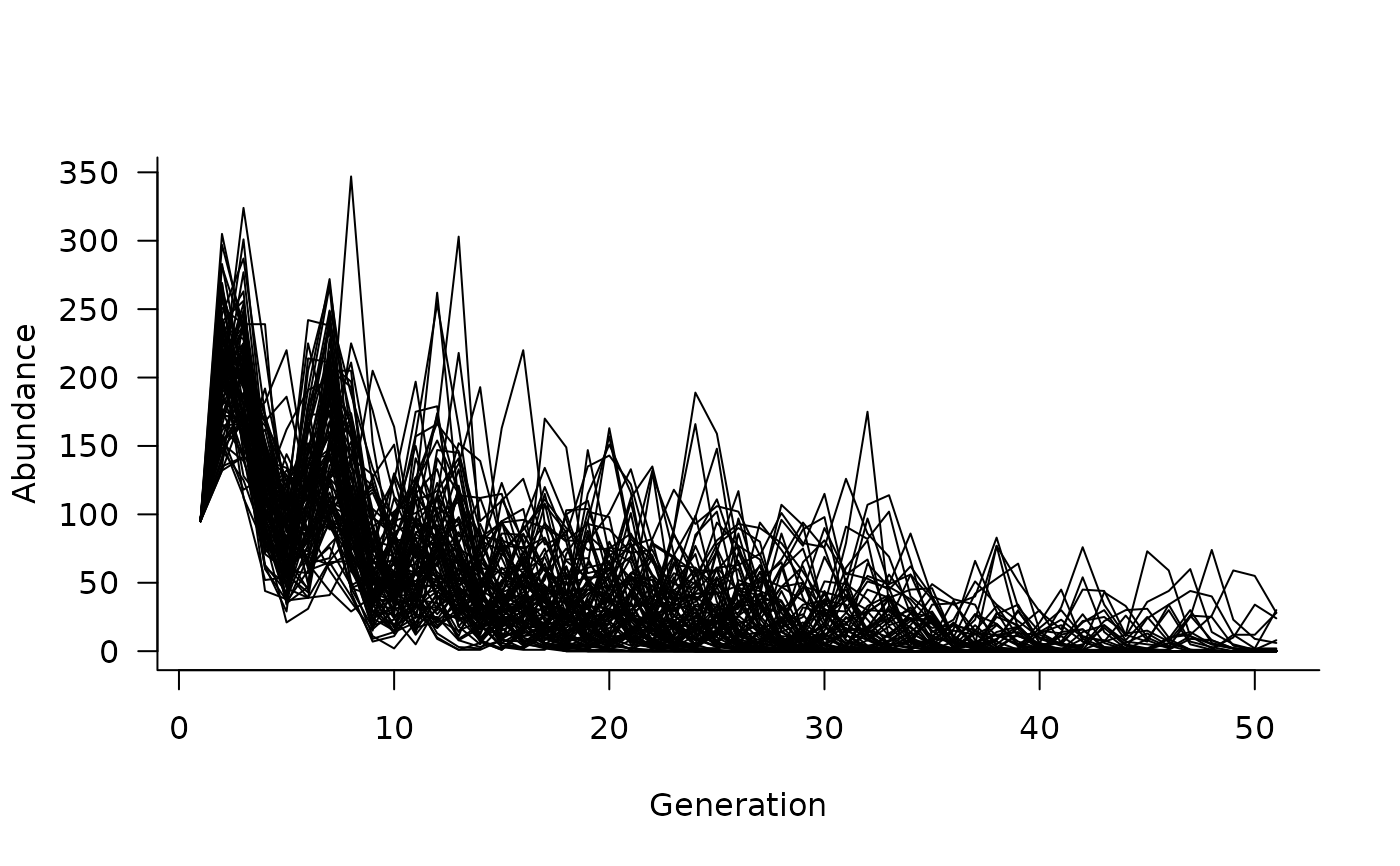
# simulate from this (50 time steps, 100 replicates)
sims <- simulate(dyn, nsim = 100, options = list(ntime = 50))

# plot the simulated trajectories
plot(sims)


# add some density dependence
dd <- density_dependence(
  masks = reproduction(popmat, dims = 4:5),
  funs = ricker(1000)
)

# update the dynamics object
dyn <- update(dyn, dd)

# simulate again
sims <- simulate(dyn, nsim = 100, options = list(ntime = 50))

# and plot
plot(sims)


# what if we want to add initial conditions?
sims <- simulate(
  dyn,
  init = c(50, 20, 10, 10, 5),
  nsim = 100,
  options = list(ntime = 50),
)

# and plot again
plot(sims)


if (FALSE) { # \dontrun{
# note that there is only one trajectory now because
#   this simulation is deterministic.
#
# let's change that by adding some environmental stochasticity
envstoch <- environmental_stochasticity(
  masks = list(
    reproduction(popmat, dims = 4:5),
    transition(popmat)
  ),
  funs = list(
    function(x) rpois(n = length(x), lambda = x),
    function(x) rmultiunit(n = 1, mean = x, sd = 0.1 * x)
  )
)

# update the dynamics object and simulate from it
dyn <- update(dyn, envstoch)
sims <- simulate(
  dyn,
  init = c(50, 20, 10, 10, 5),
  nsim = 100,
  options = list(ntime = 50),
)

# the rmultiunit draws can be slow but we can speed
#   this up by calculating them once per generation
#   instead of once per replicate within each generation
envstoch <- environmental_stochasticity(
  masks = list(
    reproduction(popmat, dims = 4:5),
    transition(popmat)
  ),
  funs = list(
    function(x, ...) rpois(n = length(x), lambda = x),
    function(x, mean, sd) {
      pnorm(mean + sd * rnorm(length(x)))
    }
  )
)

# this requires an argument "function" that takes the
#   current state of the population model in each
#   iteration and calculates the correct arguments to
#   pass to environmental_stochasticty
envstoch_function <- function(obj, pop, iter) {
  mat <- obj$matrix
  if (is.list(mat)) {
    mat <- mat[[iter]]
  }
  out <- aae.pop:::unit_to_real(
    mat[transition(mat)], 0.1 * mat[transition(mat)]
  )
  list(mean = out[, 1], sd = out[, 2])
}

# update the dynamics object and simulate from it
dyn <- update(dyn, envstoch)
sims <- simulate(
  dyn,
  init = c(50, 20, 10, 10, 5),
  nsim = 100,
  args = list(environmental_stochasticity = list(envstoch_function)),
  options = list(ntime = 50),
)

# can also add covariates that influence vital rates
#   e.g., a logistic function
covars <- covariates(
  masks = transition(popmat),
  funs = function(mat, x) mat * (1 / (1 + exp(-10 * x)))
)

# simulate 50 random covariate values
xvals <- matrix(runif(50), ncol = 1)

# update the dynamics object and simulate from it.
#   Note that ntime is now captured in the 50 values
#   of xvals, assuming we pass xvals as an argument
#   to the covariates functions
dyn <- update(dyn, covars)
sims <- simulate(
  dyn,
  init = c(50, 20, 10, 10, 5),
  nsim = 100,
  args = list(
    covariates = format_covariates(xvals),
    environmental_stochasticity = list(envstoch_function)
  )
)

# and can plot these again
plot(sims)

# a simple way to add demographic stochasticity is to change
#   the "updater" that converts the population at time t
#   to its value at time t + 1. The default in aae.pop
#   uses matrix multiplication of the vital rates matrix
#   and current population. A simple tweak is to update
#   with binomial draws. Note that this also requires a
#   change to the "tidy_abundances" option so that population
#   abundances are always integer values.
sims <- simulate(
  dyn,
  init = c(50, 20, 10, 10, 5),
  nsim = 100,
  options = list(
    update = update_binomial_leslie,
    tidy_abundances = floor
  ),
  args = list(
    covariates = format_covariates(xvals),
    environmental_stochasticity = list(envstoch_function)
  )
)

# and can plot these again
plot(sims)
} # }